Geometric Brownian Motion

Stochastic modeling of asset prices

An introduction to Geometric Brownian Motion (GBM), the foundation of modern option pricing and Monte Carlo simulation.

1 Abstract

Geometric Brownian Motion (GBM) is a continuous-time stochastic process used to model stock prices. It forms the foundation of the Black-Scholes option pricing model and assumes that prices follow a random walk consistent with the weak-form efficient market hypothesis.

2 Definition

The stochastic differential equation (SDE) for GBM is:

\[ dS = \mu S \, dt + \sigma S \, dW \]

Where:

• \(S\) = asset price
• \(\mu\) = drift (expected return)
• \(\sigma\) = volatility (standard deviation of returns)
• \(dW\) = Wiener process (standard Brownian motion)

3 Discrete Form

For simulation purposes, we use the discrete approximation:

\[ \frac{\Delta S}{S} = \mu \Delta t + \sigma \varepsilon \sqrt{\Delta t} \]

Where \(\varepsilon \sim N(0,1)\) is a standard normal random variable.

The first term (\(\mu \Delta t\)) is the drift — the expected directional movement. The second term (\(\sigma \varepsilon \sqrt{\Delta t}\)) is the shock — random fluctuation scaled by volatility.

4 Analytical Solution

The exact solution to the GBM SDE is:

\[ S(t) = S_0 \exp\left[\left(\mu - \frac{\sigma^2}{2}\right)t + \sigma W(t)\right] \]

This shows that prices are log-normally distributed (always positive), while returns are normally distributed.

5 Simulation (Python)

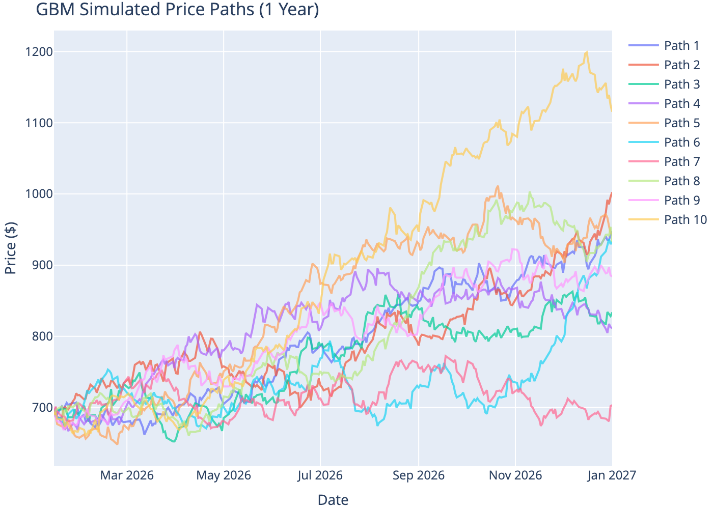
We simulate 10 possible price paths for a stock over 1 year using historical SPY parameters.

Initial Price: $689.42
Annual Drift (μ): 19.97%
Annual Volatility (σ): 16.26%

	Path 1	Path 2	Path 3	Path 4	Path 5	Path 6	Path 7	Path 8	Path 9	Path 10
2026-12-28	940.351636	973.706233	816.717561	810.539100	971.258809	919.331363	684.347186	942.733507	888.400176	1155.844317
2026-12-29	935.224328	991.745409	834.179546	804.792609	966.520387	928.150647	682.142788	942.992669	889.289266	1134.171455
2026-12-30	935.784102	985.490683	830.590012	817.389824	954.863551	936.609321	680.699478	940.989754	897.183859	1138.972658
2026-12-31	941.968091	996.052310	828.388203	812.879866	945.004999	929.409366	702.101015	953.772625	885.504854	1124.475841
2027-01-01	947.331151	1002.394747	833.676855	811.359486	944.489876	933.227374	703.239482	933.020007	884.076480	1115.534543

6 Simulated Price Paths

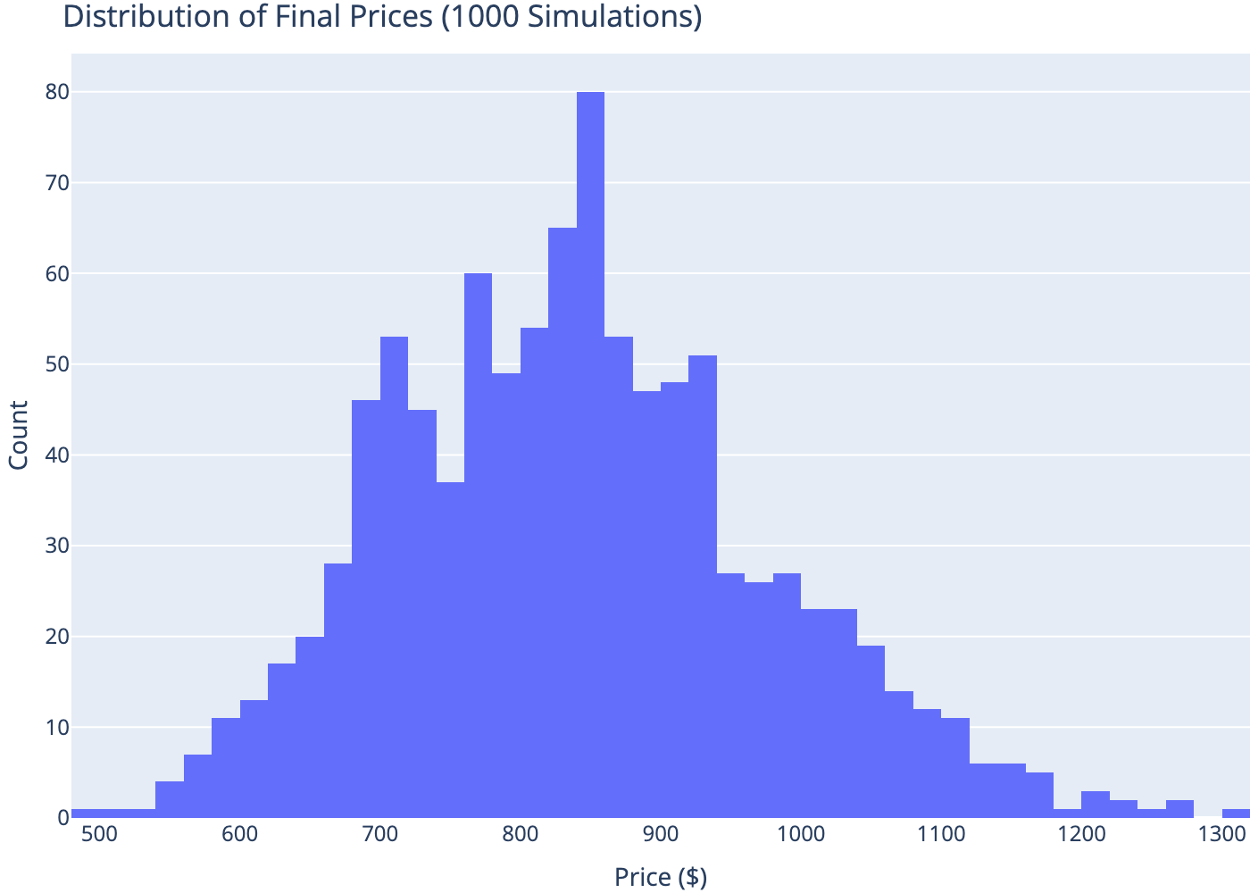
7 Distribution of Final Prices

8 Conclusion

Geometric Brownian Motion provides a mathematically tractable model for asset prices. While it has limitations (assumes constant volatility and continuous trading), GBM remains fundamental to quantitative finance for option pricing, risk management, and Monte Carlo simulation.