GARCH Models

Modeling volatility clustering

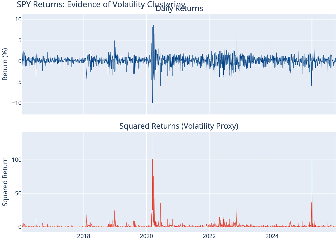
GARCH models capture volatility clustering—the tendency for large price moves to follow large moves and small moves to follow small moves.

1 Abstract

The Generalized Autoregressive Conditional Heteroskedasticity (GARCH) model, introduced by Bollerslev (1986), captures a key empirical feature of financial returns: volatility clustering. Large price movements tend to cluster together, as do small movements. GARCH models allow volatility to vary over time, improving risk forecasts and option pricing.

2 Volatility Clustering

Financial returns exhibit:

• Volatility clustering: High volatility periods followed by high volatility
• Fat tails: More extreme returns than normal distribution predicts
• Leverage effect: Negative returns often increase volatility more than positive returns

3 GARCH(1,1) Model

The standard GARCH(1,1) model:

Return equation: \[ r_t = \mu + \varepsilon_t, \quad \varepsilon_t = \sigma_t z_t, \quad z_t \sim N(0,1) \]

Variance equation: \[ \sigma_t^2 = \omega + \alpha \varepsilon_{t-1}^2 + \beta \sigma_{t-1}^2 \]

Where:

• \(\omega > 0\) = constant (base variance)
• \(\alpha \geq 0\) = ARCH coefficient (shock impact)
• \(\beta \geq 0\) = GARCH coefficient (persistence)
• \(\alpha + \beta < 1\) for stationarity

4 Interpretation

• \(\alpha\): How much recent shocks affect current volatility
• \(\beta\): How persistent volatility is over time
• \(\alpha + \beta\): Overall persistence (close to 1 = highly persistent)
• Long-run variance: \(\bar{\sigma}^2 = \frac{\omega}{1 - \alpha - \beta}\)

5 Compute (Python)

Sample size: 2514 observations
Mean return: 0.0575%
Std deviation: 1.1336%

6 Evidence of Volatility Clustering

7 Fit GARCH(1,1) Model

                     Constant Mean - GARCH Model Results                      
==============================================================================
Dep. Variable:                  Close   R-squared:                       0.000
Mean Model:             Constant Mean   Adj. R-squared:                  0.000
Vol Model:                      GARCH   Log-Likelihood:               -3221.16
Distribution:                  Normal   AIC:                           6450.32
Method:            Maximum Likelihood   BIC:                           6473.63
                                        No. Observations:                 2514
Date:                Wed, Jan 14 2026   Df Residuals:                     2513
Time:                        21:46:56   Df Model:                            1
                                Mean Model                                
==========================================================================
                 coef    std err          t      P>|t|    95.0% Conf. Int.
--------------------------------------------------------------------------
mu             0.0914  1.464e-02      6.241  4.335e-10 [6.270e-02,  0.120]
                              Volatility Model                              
============================================================================
                 coef    std err          t      P>|t|      95.0% Conf. Int.
----------------------------------------------------------------------------
omega          0.0379  1.029e-02      3.684  2.295e-04 [1.775e-02,5.811e-02]
alpha[1]       0.1813  3.032e-02      5.979  2.249e-09     [  0.122,  0.241]
beta[1]        0.7899  2.973e-02     26.572 1.447e-155     [  0.732,  0.848]
============================================================================

Covariance estimator: robust

8 Extract Parameters

Long-run daily variance: 1.3172
Long-run annualized volatility: 18.22%

	Parameter	Value
0	μ (mean)	0.091403
1	ω (omega)	0.037928
2	α (alpha)	0.181284
3	β (beta)	0.789923
4	α + β	0.971207

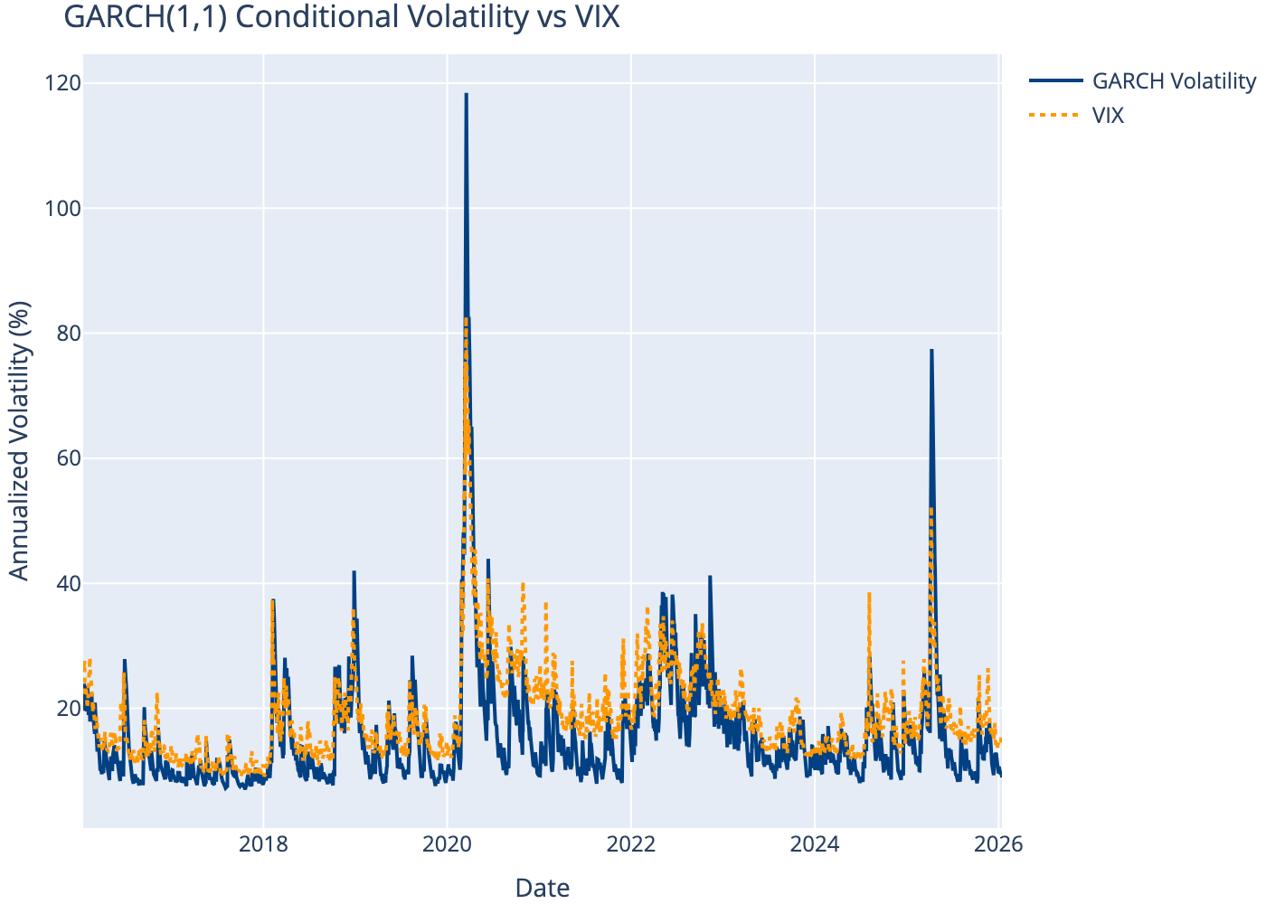
9 Conditional Volatility

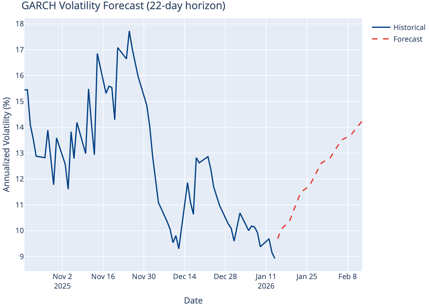
10 Volatility Forecast

11 Model Comparison

Compare different GARCH specifications.

	Model	Log-Likelihood	AIC	BIC
0	GARCH(1,1)	-3221.16	6450.32	6473.63
1	GARCH(2,1)	-3221.14	6452.29	6481.44
2	EGARCH(1,1)	-3231.61	6471.23	6494.55
3	GJR-GARCH(1,1)	-3189.03	6388.06	6417.20

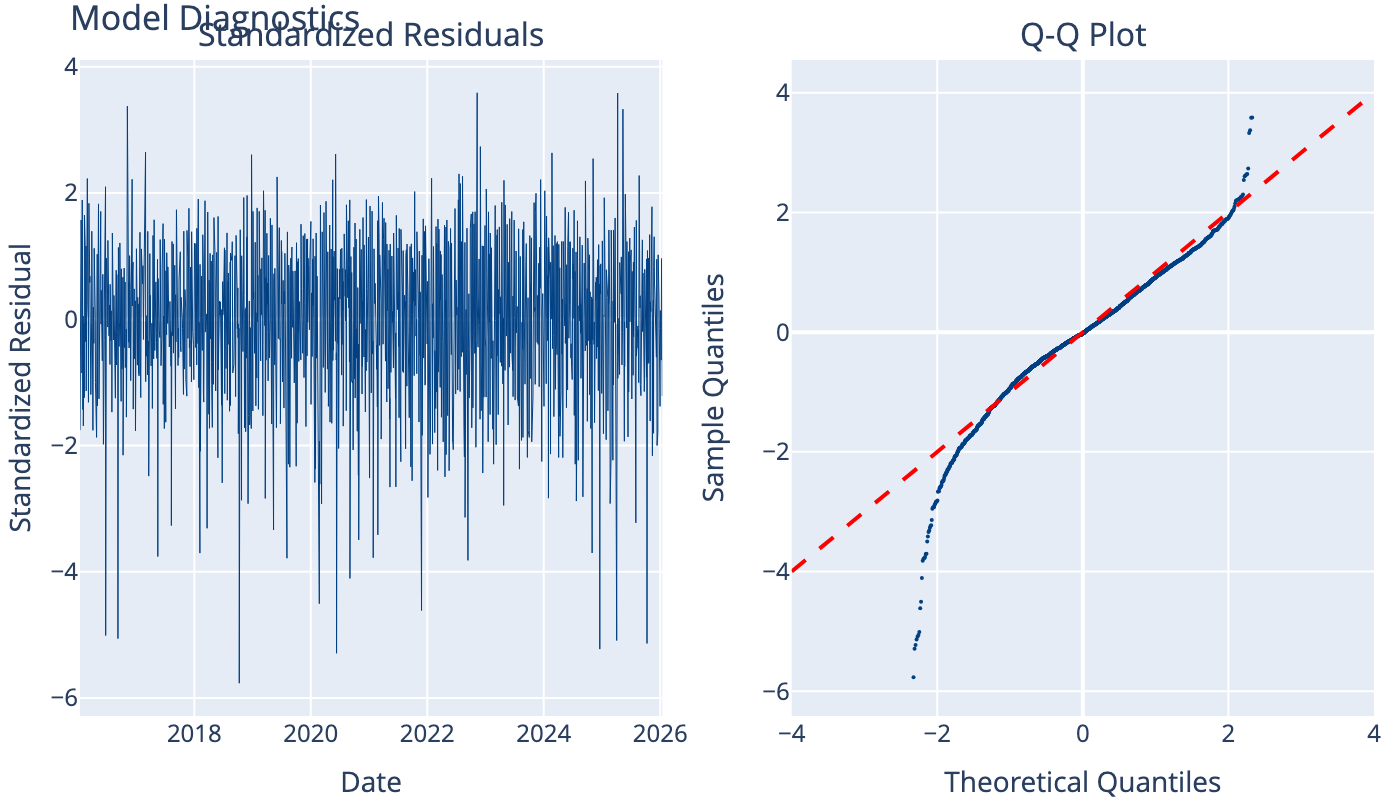
12 Standardized Residuals

Check if the model captures volatility dynamics properly.

13 Applications

1. Value at Risk (VaR): Time-varying volatility improves risk estimates
2. Option Pricing: Better volatility forecasts improve pricing
3. Portfolio Optimization: Dynamic allocation based on volatility regimes
4. Trading: Volatility mean reversion strategies

14 Conclusion

GARCH models capture the empirical reality that volatility is not constant but varies predictably over time. The GARCH(1,1) model is often sufficient for most applications, with extensions like EGARCH and GJR-GARCH capturing additional features like the leverage effect. Volatility forecasts from GARCH models are widely used in risk management, option pricing, and trading strategies.