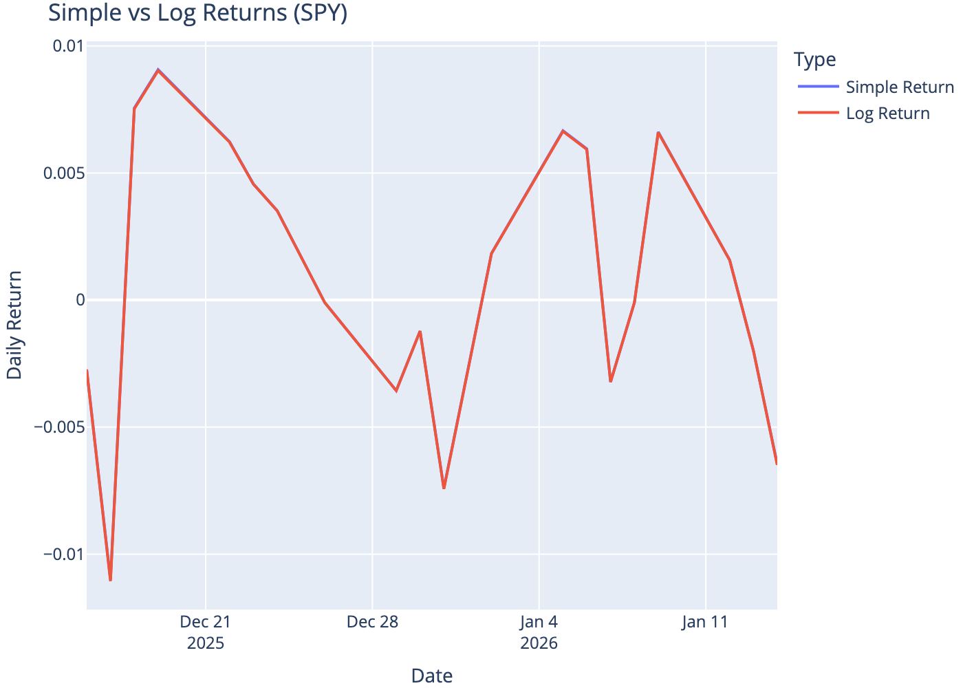
| Price | Close | Simple Return | Log Return |
|---|---|---|---|
| Date | |||
| 2025-12-31 | 681.92 | -0.0074 | -0.0074 |
| 2026-01-02 | 683.17 | 0.0018 | 0.0018 |
| 2026-01-05 | 687.72 | 0.0067 | 0.0066 |
| 2026-01-06 | 691.81 | 0.0059 | 0.0059 |
| 2026-01-07 | 689.58 | -0.0032 | -0.0032 |
| 2026-01-08 | 689.51 | -0.0001 | -0.0001 |
| 2026-01-09 | 694.07 | 0.0066 | 0.0066 |
| 2026-01-12 | 695.16 | 0.0016 | 0.0016 |
| 2026-01-13 | 693.77 | -0.0020 | -0.0020 |
| 2026-01-14 | 689.28 | -0.0065 | -0.0065 |
Returns
Measuring investment performance
1 Abstract
A return is a profit or loss on an investment over a particular time period. Positive returns indicate profit, negative returns indicate loss. Returns allow comparison of performance across different investments regardless of their absolute price.
2 Simple Return
The simple (arithmetic) return is calculated as:
\[ R_t = \frac{P_t - P_{t-1}}{P_{t-1}} = \frac{P_t}{P_{t-1}} - 1 \]
Where \(P_t\) is the price at time \(t\) and \(P_{t-1}\) is the previous price.
Example: Buy at $1000, sell at $1200
\[ R = \frac{1200 - 1000}{1000} = 0.20 = 20\% \]
If the price drops to $800 instead:
\[ R = \frac{800 - 1000}{1000} = -0.20 = -20\% \]
3 Log Return
In quantitative finance, logarithmic returns are preferred:
\[ r_t = \ln\left(\frac{P_t}{P_{t-1}}\right) = \ln(P_t) - \ln(P_{t-1}) \]
Why log returns?
- Time additivity: Multi-period log returns sum directly: \(r_{total} = r_1 + r_2 + ... + r_n\)
- Statistical properties: More likely to be normally distributed
- Symmetry: +10% and -10% log returns are symmetric around zero
4 Compute (Python)
5 Comparison

6 Conclusion
Simple returns are intuitive for single-period calculations, but log returns are preferred in quantitative finance due to their time-additive property and better statistical behavior. For small returns, simple and log returns are approximately equal.