| Ticker | EEM | EFA | GLD | IWM | QQQ | SPY | TLT | VNQ |
|---|---|---|---|---|---|---|---|---|
| Ticker | ||||||||
| EEM | 1.00 | 0.79 | 0.30 | 0.65 | 0.67 | 0.68 | 0.06 | 0.48 |
| EFA | 0.79 | 1.00 | 0.29 | 0.75 | 0.73 | 0.81 | 0.10 | 0.64 |
| GLD | 0.30 | 0.29 | 1.00 | 0.14 | 0.11 | 0.13 | 0.24 | 0.20 |
| IWM | 0.65 | 0.75 | 0.14 | 1.00 | 0.76 | 0.84 | 0.07 | 0.71 |
| QQQ | 0.67 | 0.73 | 0.11 | 0.76 | 1.00 | 0.95 | 0.08 | 0.56 |
| SPY | 0.68 | 0.81 | 0.13 | 0.84 | 0.95 | 1.00 | 0.06 | 0.69 |
| TLT | 0.06 | 0.10 | 0.24 | 0.07 | 0.08 | 0.06 | 1.00 | 0.26 |
| VNQ | 0.48 | 0.64 | 0.20 | 0.71 | 0.56 | 0.69 | 0.26 | 1.00 |
Correlation
Measuring asset co-movement
finance
basics
portfolio
Correlation measures how assets move together, fundamental to portfolio diversification and risk management.
1 Abstract
Correlation measures the linear relationship between two variables. In finance, asset correlations determine diversification benefits — low or negative correlations reduce portfolio risk. However, correlations are unstable and often increase during market stress, precisely when diversification is most needed.
2 Definition
The Pearson correlation coefficient between assets \(X\) and \(Y\) is:
\[ \rho_{X,Y} = \frac{\text{Cov}(X, Y)}{\sigma_X \sigma_Y} = \frac{E[(X - \mu_X)(Y - \mu_Y)]}{\sigma_X \sigma_Y} \]
Where:
- \(\text{Cov}(X, Y)\) = covariance between \(X\) and \(Y\)
- \(\sigma_X, \sigma_Y\) = standard deviations
- \(\mu_X, \mu_Y\) = means
The correlation coefficient ranges from \(-1\) to \(+1\):
| Value | Interpretation |
|---|---|
| +1 | Perfect positive correlation |
| 0 | No linear relationship |
| -1 | Perfect negative correlation |
3 Covariance Matrix
For a portfolio of \(n\) assets, the covariance matrix \(\Sigma\) captures all pairwise relationships:
\[ \Sigma = \begin{bmatrix} \sigma_1^2 & \sigma_{1,2} & \cdots & \sigma_{1,n} \\ \sigma_{2,1} & \sigma_2^2 & \cdots & \sigma_{2,n} \\ \vdots & \vdots & \ddots & \vdots \\ \sigma_{n,1} & \sigma_{n,2} & \cdots & \sigma_n^2 \end{bmatrix} \]
The correlation matrix normalizes this by the standard deviations.
4 Compute (Python)
5 Correlation Heatmap
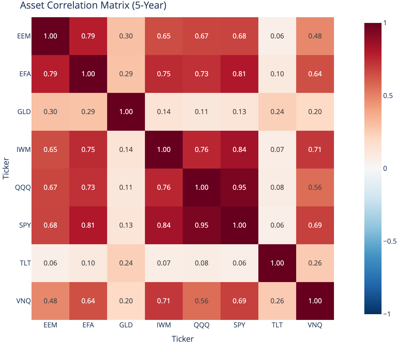
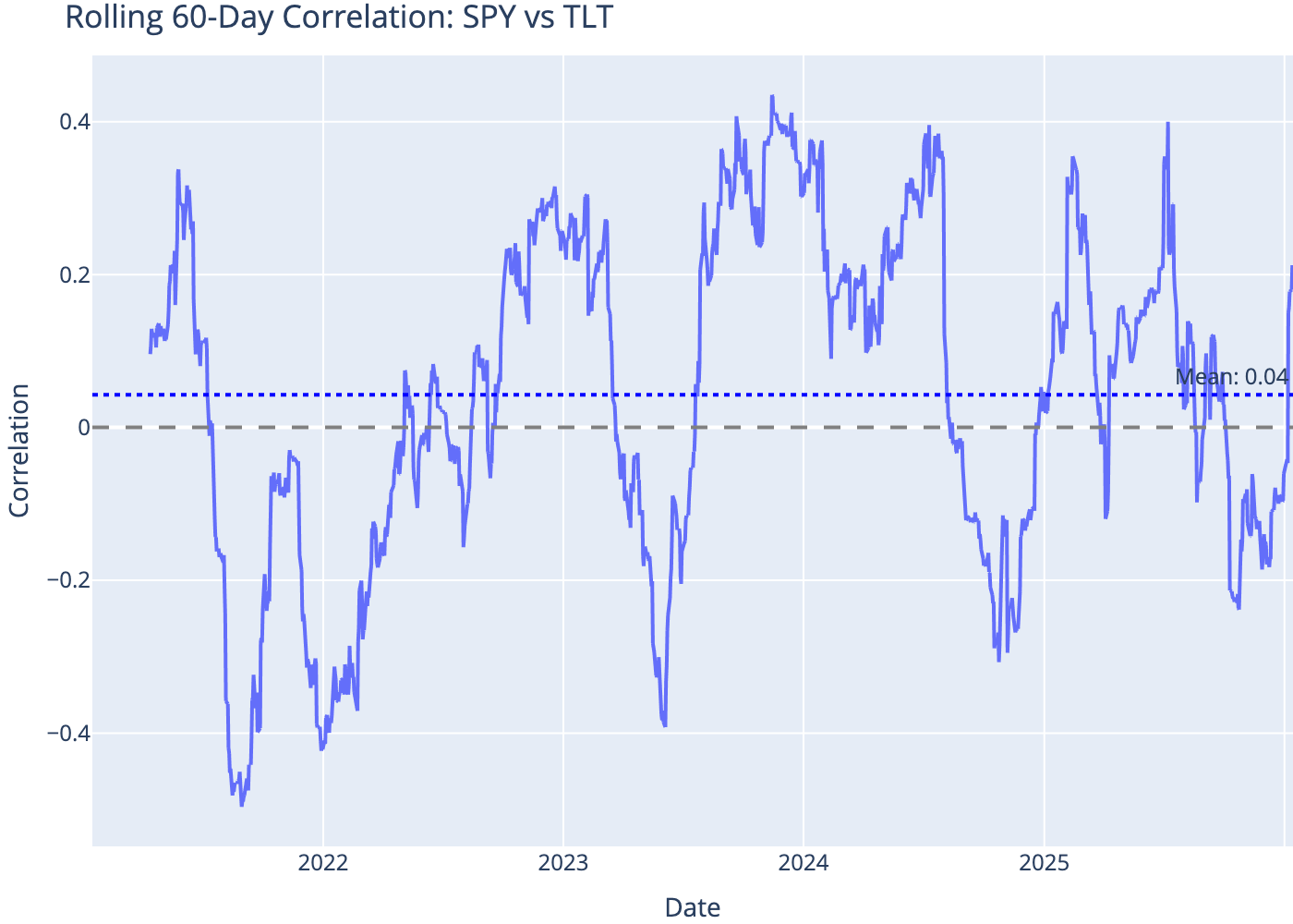
6 Rolling Correlation
Correlations change over time, especially during market stress.
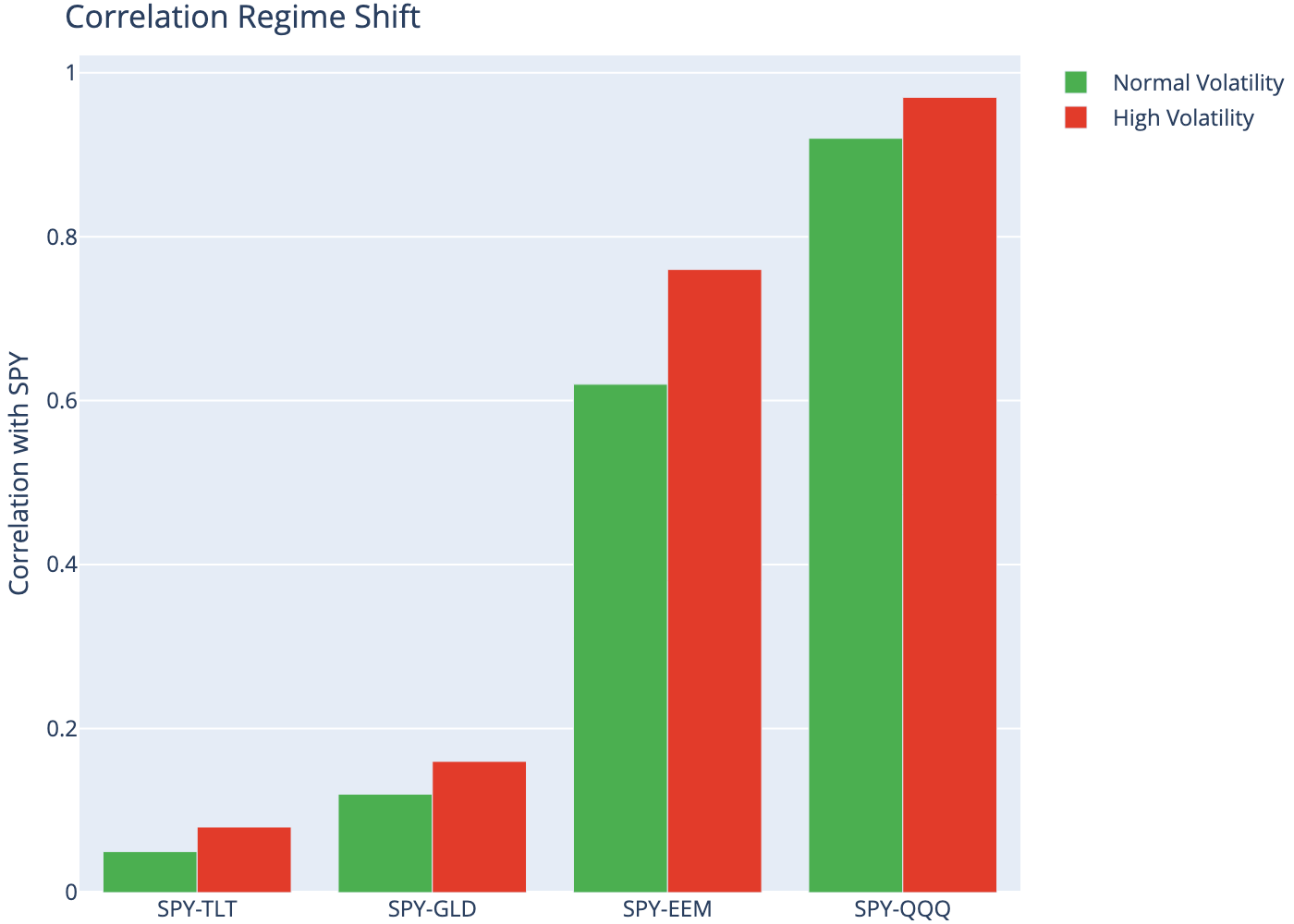
7 Correlation During Stress
Correlations tend to spike during market downturns — the “correlation breakdown” problem.
| Asset Pair | Normal Vol | High Vol | Change | |
|---|---|---|---|---|
| 0 | SPY-TLT | 0.05 | 0.08 | 0.03 |
| 1 | SPY-GLD | 0.12 | 0.16 | 0.04 |
| 2 | SPY-EEM | 0.62 | 0.76 | 0.14 |
| 3 | SPY-QQQ | 0.92 | 0.97 | 0.05 |
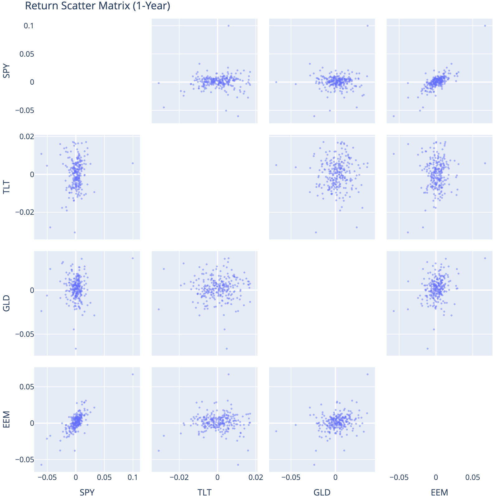
8 Scatter Plot Matrix
Visualize pairwise relationships between major asset classes.
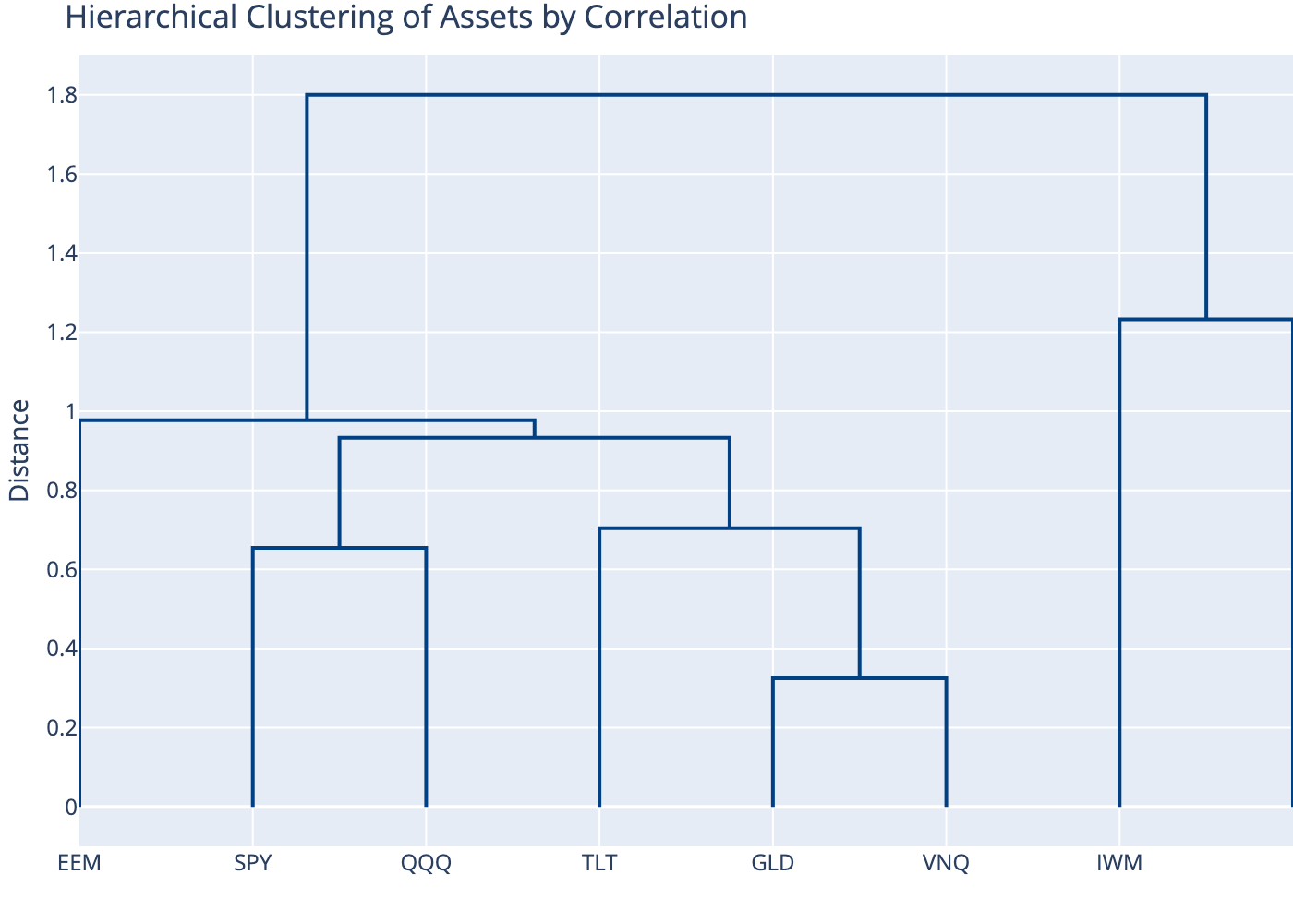
9 Hierarchical Clustering
Group assets by correlation similarity for portfolio construction.
10 Limitations
- Linear only: Correlation misses non-linear dependencies
- Unstable: Changes significantly over time and across regimes
- Not causation: Correlation does not imply one asset causes another to move
- Outlier sensitive: Extreme values can distort correlation estimates
11 Conclusion
Correlation is fundamental to portfolio construction and risk management. While low correlations improve diversification, investors must recognize that correlations are unstable and tend to increase during market stress. Rolling correlation analysis and regime-conditional estimates provide more realistic inputs for portfolio optimization.