Mean-Variance Optimization

Markowitz portfolio theory

Mean-variance optimization finds the portfolio weights that maximize return for a given risk level, forming the efficient frontier.

1 Abstract

Mean-variance optimization (MVO), introduced by Harry Markowitz in 1952, is the foundational framework of modern portfolio theory. It finds optimal portfolio weights by maximizing expected return for a given level of risk, or equivalently, minimizing risk for a given return target. The set of optimal portfolios forms the efficient frontier.

2 Definition

For a portfolio of \(n\) assets with weight vector \(\mathbf{w}\):

Portfolio return: \[ \mu_p = \mathbf{w}^T \boldsymbol{\mu} \]

Portfolio variance: \[ \sigma_p^2 = \mathbf{w}^T \Sigma \mathbf{w} \]

Where:

• \(\boldsymbol{\mu}\) = vector of expected returns
• \(\Sigma\) = covariance matrix
• \(\mathbf{w}\) = weight vector with \(\sum w_i = 1\)

3 Optimization Problem

Minimum variance for target return \(\mu^*\):

\[ \min_{\mathbf{w}} \quad \mathbf{w}^T \Sigma \mathbf{w} \]

Subject to: \[ \mathbf{w}^T \boldsymbol{\mu} = \mu^* \quad \text{(return target)} \] \[ \mathbf{w}^T \mathbf{1} = 1 \quad \text{(fully invested)} \] \[ w_i \geq 0 \quad \text{(no short selling, optional)} \]

4 Compute (Python)

Expected Annual Returns:
Ticker
EFA    0.0859
GLD    0.1800
SPY    0.1343
TLT   -0.0771
VNQ    0.0532
dtype: float64

Covariance Matrix:
Ticker     EFA     GLD     SPY     TLT     VNQ
Ticker                                        
EFA     0.0256  0.0072  0.0220  0.0026  0.0194
GLD     0.0072  0.0243  0.0034  0.0060  0.0059
SPY     0.0220  0.0034  0.0291  0.0017  0.0222
TLT     0.0026  0.0060  0.0017  0.0257  0.0079
VNQ     0.0194  0.0059  0.0222  0.0079  0.0355

5 Portfolio Optimization Functions

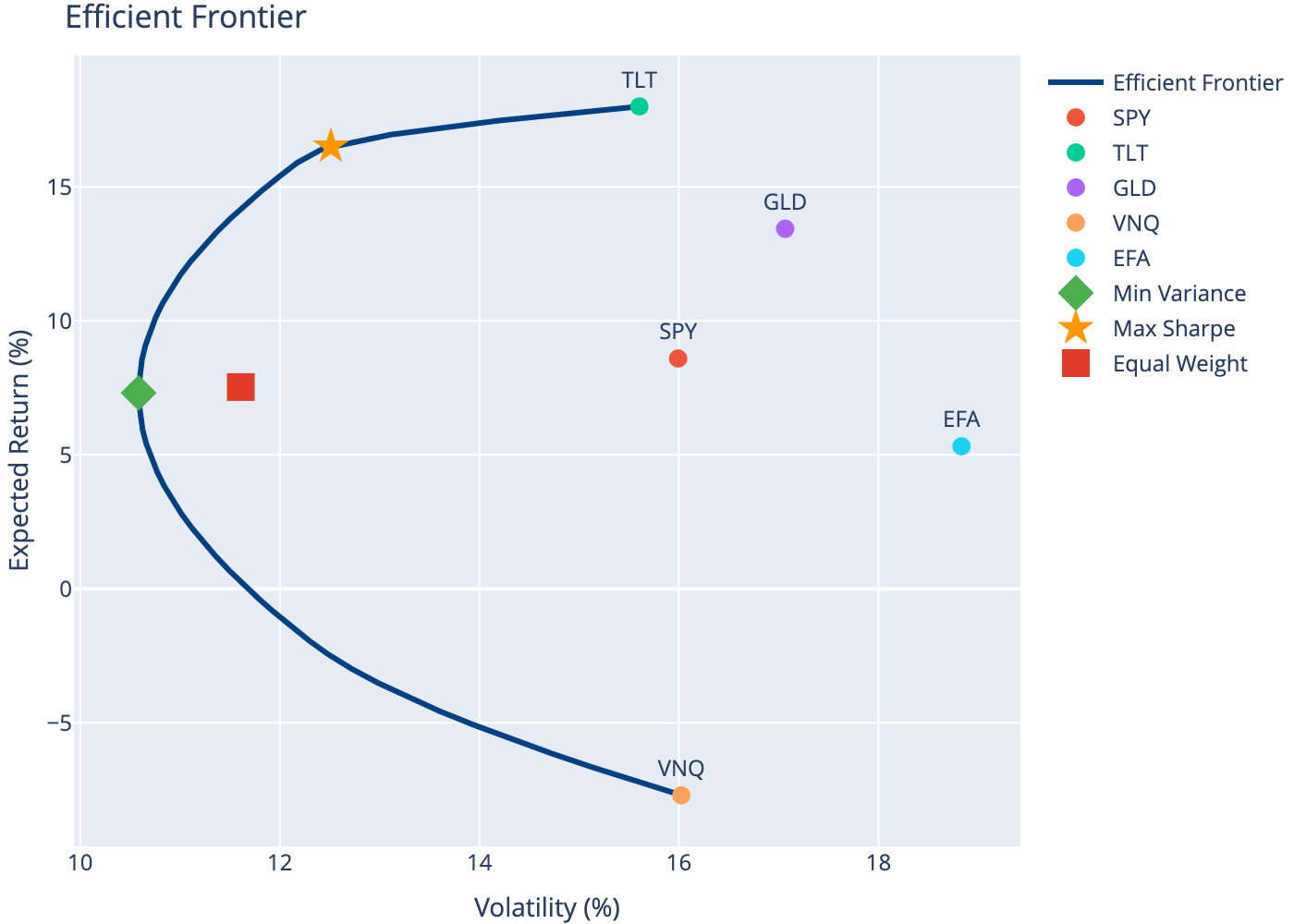
6 Efficient Frontier

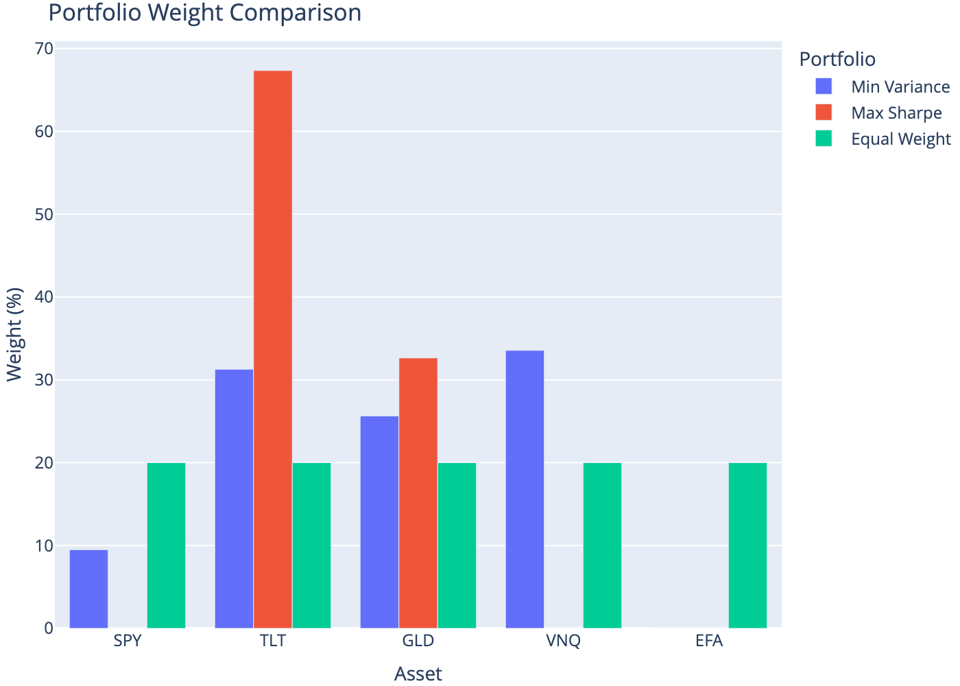
7 Optimal Portfolio Weights

	Asset	Min Variance	Max Sharpe	Equal Weight
0	SPY	9.50	0.00	20.0
1	TLT	31.29	67.35	20.0
2	GLD	25.65	32.65	20.0
3	VNQ	33.56	0.00	20.0
4	EFA	0.00	0.00	20.0

8 Portfolio Statistics

	Portfolio	Return (%)	Volatility (%)	Sharpe Ratio
0	Min Variance	7.31	10.58	0.31
1	Max Sharpe	16.51	12.51	1.00
2	Equal Weight	7.53	11.61	0.30

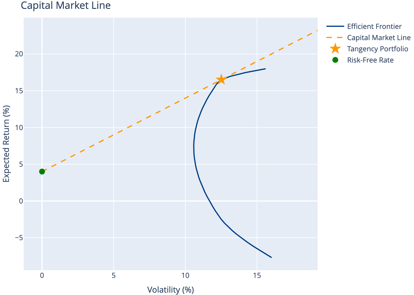
9 Capital Market Line

With a risk-free asset, investors can combine the tangency portfolio (max Sharpe) with borrowing/lending at the risk-free rate.

10 Limitations

• Estimation error: Small changes in inputs cause large weight changes
• Concentrated portfolios: Often produces extreme allocations
• Historical data: Past returns don’t predict future returns
• Single period: Ignores rebalancing and transaction costs
• Normal assumption: Doesn’t account for fat tails or skewness

Modern approaches like Black-Litterman, shrinkage estimators, and robust optimization address some of these limitations.

11 Conclusion

Mean-variance optimization provides the theoretical foundation for portfolio construction. While the basic framework has practical limitations, understanding MVO is essential for quantitative finance. The efficient frontier demonstrates the fundamental risk-return tradeoff, and the capital market line shows how combining a risk-free asset with the tangency portfolio improves investment opportunities.