Value at Risk

Quantifying potential losses

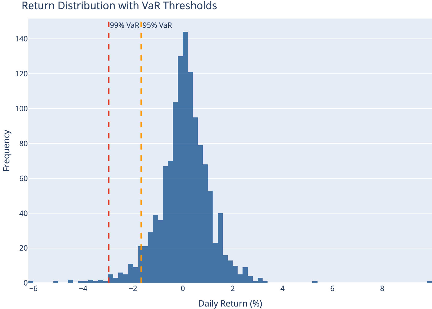
Value at Risk (VaR) estimates the maximum loss over a given time horizon at a specified confidence level.

1 Abstract

Value at Risk (VaR) answers a simple question: “What is my maximum expected loss over a given period at a given confidence level?” For example, a 1-day 95% VaR of $1 million means there’s a 5% chance of losing more than $1 million in one day. VaR became a regulatory standard after the 1996 Basel Accord.

2 Definition

The VaR at confidence level \(\alpha\) is the \(\alpha\)-quantile of the loss distribution:

\[ P(L \leq VaR_\alpha) = \alpha \]

Equivalently, for returns:

\[ VaR_\alpha = -\mu - \sigma \cdot z_\alpha \]

Where \(z_\alpha\) is the \(\alpha\)-quantile of the standard normal distribution.

Common parameters:

• Confidence: 95% (\(z = 1.645\)) or 99% (\(z = 2.326\))
• Horizon: 1-day, 10-day (regulatory), or longer

3 VaR Methods

1. Parametric (Variance-Covariance): Assumes normal distribution
2. Historical Simulation: Uses actual historical returns
3. Monte Carlo: Simulates many scenarios

4 Compute (Python)

Portfolio Value: $1,000,000
Sample Period: 2021-01-15 to 2026-01-14
Mean Daily Return: 0.0533%
Daily Volatility: 1.0750%

5 Method 1: Parametric VaR

Assumes returns follow a normal distribution.

	Confidence	VaR (%)	VaR ($)
0	90%	1.32	13243.18
1	95%	1.71	17148.62
2	99%	2.45	24474.58

6 Method 2: Historical Simulation

Uses actual historical returns without distributional assumptions.

	Confidence	VaR (%)	VaR ($)
0	90%	1.18	11830.60
1	95%	1.68	16757.72
2	99%	2.97	29724.75

7 Method 3: Monte Carlo VaR

Simulates many scenarios using estimated parameters.

	Confidence	VaR (%)	VaR ($)
0	90%	1.34	13358.72
1	95%	1.73	17256.17
2	99%	2.44	24412.17

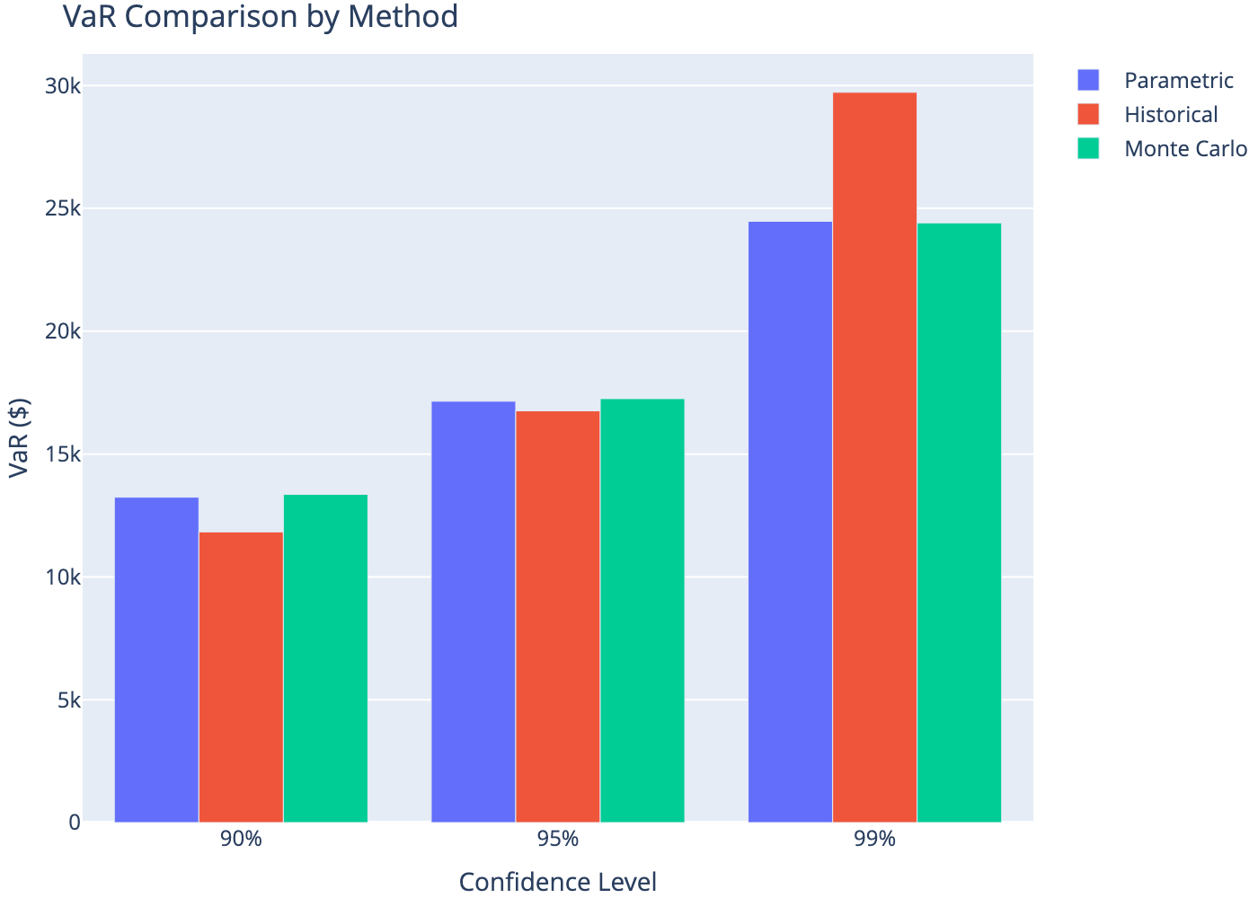
8 Method Comparison

	Confidence	Parametric	Historical	Monte Carlo
0	90%	13243.0	11831.0	13359.0
1	95%	17149.0	16758.0	17256.0
2	99%	24475.0	29725.0	24412.0

9 VaR Visualization

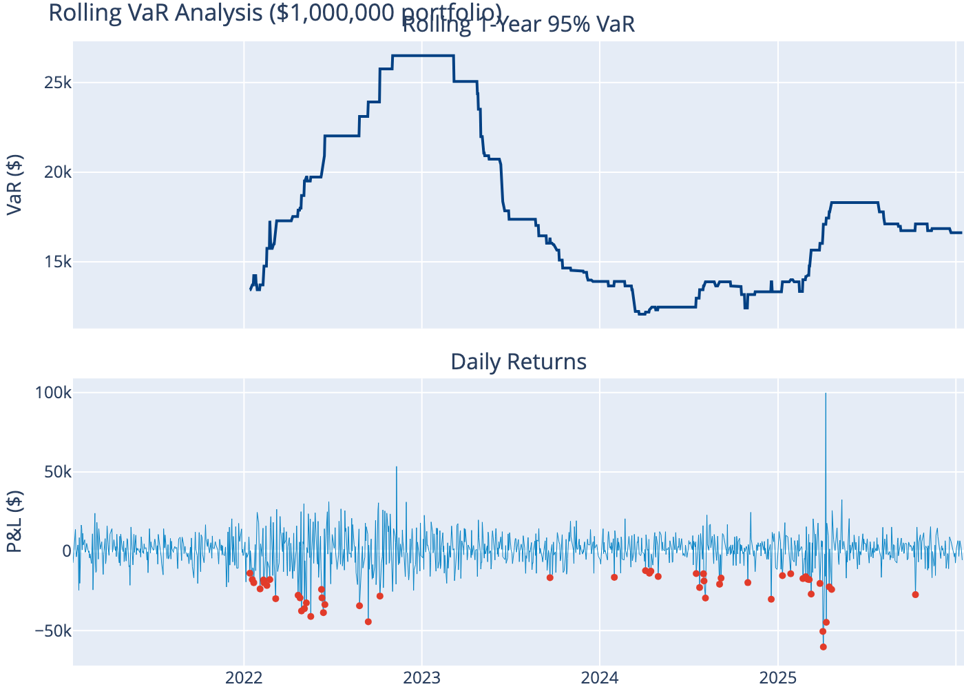
10 Rolling VaR

VaR changes over time as market conditions evolve.

11 VaR Backtesting

Check how often actual losses exceed VaR predictions.

Expected Exception Rate: 5.00%
Actual Exception Rate: 4.06%
Number of Exceptions: 51
Total Observations: 1255

Kupiec Test p-value: 0.9474
VaR Model Valid (p > 0.05): Yes

12 Expected Shortfall (CVaR)

VaR tells you the threshold; Expected Shortfall (ES) tells you the average loss when that threshold is breached.

\[ ES_\alpha = E[L | L > VaR_\alpha] \]

	Confidence	VaR ($)	ES ($)	ES/VaR
0	90%	11831.0	19608.0	2.0
1	95%	16758.0	25159.0	2.0
2	99%	29725.0	39588.0	1.0

13 Limitations

• Not coherent: VaR can penalize diversification
• Ignores tail shape: Doesn’t tell you how bad losses can get beyond VaR
• Assumption-dependent: Parametric VaR assumes normal distribution
• Backward-looking: Historical VaR may miss structural changes

14 Conclusion

VaR provides a simple, intuitive risk metric that has become industry standard. However, it should be complemented with Expected Shortfall for tail risk and stress testing for extreme scenarios. The choice of method (parametric, historical, or Monte Carlo) depends on the portfolio complexity and distributional assumptions. Regular backtesting ensures the VaR model remains valid over time.